Two (of Three) Ways of Looking at C19 Newspaper Exchange Networks
I wrote the following as part of my preparation for next week’s second meeting of the NHC Summer Institute in Digital Textual Studies next week. The post assumes a modest working understanding of network graphs and their terminology. For a primer on humanities network analysis, see the links for my network analysis workshop or, more specifically, see Scott Weingart’s ongoing series Demystifying Networks, beginning, appropriately enough with his introduction, his second post about degree, and possibly his post on communities.
Introduction
In previous work in American Literary History, I argued that reprinted nineteenth-century newspaper selections should be considered as authored by the network of periodicals exchanges. Such texts were assemblages, defined by circulation and mutability, that cannot cohere around a single, stable author. As part of this argument, I demonstrated how social network analysis (SNA) methods might employ large-scale data about reprinting to illuminate lines of influence among newspapers during the period. In that early network modeling, I represented individual newspapers from our reprinting data—at the time drawn primarily from the Library of Congress’ Chronicling America collection—as nodes, connected by edges that represented texts printed in common between papers. Those edges were weighted by frequency of shared reprints. The working assumptions behind those models were these: 1.) the fact that two newspapers reprint this or that text in common says very little about their relationship, or lack thereof, during the period and 2.) that when two newspaper printed hundreds, thousands, or even tens of thousands of texts in common, this fact is a strong signal of a potential relationship between them.
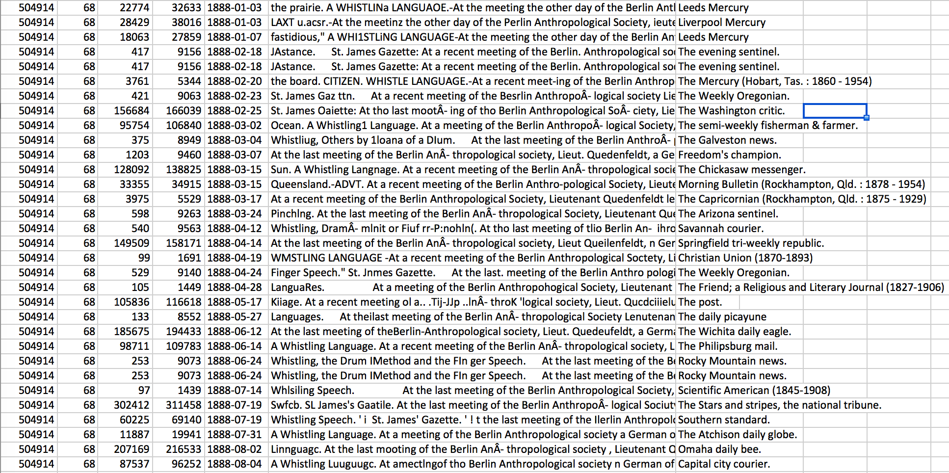
A selection from a single cluster in the Viral Data. Each line represents a specific reprint from the larger cluster, which is identified by the ID in the first column. You can browse the cluster data I used for these experiments. These are themselves experimental clusters using a new version of the reprint-detection algorithm, and are not yet suitable for formal publication.
Our data about reprinting in the Viral Texts Project is organized around “clusters”: these are, essentially, enumerative bibliographies of particular texts that circulated in nineteenth-century newspapers, derived computationally through a reprint detection algorithm that we describe more fully in previous publications.1 From these chronologically-ordered lists of witnesses, we derive network structures by tallying how often publications appear in the same clusters. When two publications appear together in a particular cluster, they are considered linked, with an edge of weight 1. Each subsequent time those same publications appear together in other clusters, the weight of their edge increases by 1; ten shared reprints results in a weight of 10, one hundred shared reprints in a weight of 100. Thus the final network data shows strong links between publications that often print the same texts and weaker links between publications that occasionally print the same texts.
This method works reasonably well for ascertaining potential lines of influence among nineteenth-century periodicals. That two newspapers happen to share a few texts in common says very little: the mechanics of nineteenth-century reprinting were dynamic and varied enough that nearly any two newspapers were bound to occasionally print the same texts, whether or not those particular newspapers had any direct or near-removed relationship. The general network model we have used to this point does assume, however, that when two newspapers share hundreds, thousands, or even tens of thousands of texts in common, these alignments can be strong indicators that allow us to hypothesize a close relationship between them. However, we cannot conclude direct influence from this network model, if only because our population of newspapers is incomplete, even fragmentary: limited to those newspapers which have been digitized and whose data we can access. Our text mining draws on several thousands of newspapers, but these represent a small fraction of the papers that would have been extant in the nineteenth century, which means there are potentially far more nodes missing from our data than nodes present. Thus we cannot draw firm conclusions directly from our network graphs; instead, we treat them as indicators which can direct more focused research. When we see a strong link between two papers in the model, this points us back to the archive to discern what the nature of that link might be: are these papers politically affiliated? Geographically close? Were their editors friends, or relatives?
This iterative process from the model to the archive and back has been enlightening and useful, though from the beginning it has been clear that refinement of our data and model are both possible and necessary. For instance, how does time play into these network models? The world of nineteenth century newspapers was incredibly volatile, with new publications constantly appearing and old ones disappearing. In addition, even ongoing papers were constantly changing their names (sometimes due to mergers or schisms), swapping their political affiliations, and sometimes even moving locations. Which is to say, we would expect the dynamics of our network model to shift dramatically over the nineteenth century as particular papers waxed and waned in influence, or as relationships among those papers shifted.
Recently, then, I have begun working to generate more nuanced network data from our reprinting evidence, taking into account a range of variables that might influence how we understand the relationships among newspapers within clusters. These variables include textual overlap, time lag, and geographical distance, measured between each possible pair of reprints within each cluster. Considering these modifications in turn, we produce not one network model, but instead multiple models of nineteenth-century newspaper network relations that can be compared and contrasted. Each network variable used for our models incorporates specific domain knowledge about the operations of nineteenth century reprinting—in other words, insights drawn from literary-historical periodicals scholarship—toward a more subtle and specific SNA for understanding historical network operations. Of course, each of these models is a simplification of the phenomena it represents, honed on a particular facet of the newspaper exchanges at the expense of others. By considering the network through multiple facets we can gain a fuller—though never complete—picture of how nineteenth century newspaper reprinting evidences historical network relationships.
The experiments that follow are just that: experiments. These are not yet polished network analyses, but attempts to push against the limitations of our initial models in intellectually generative ways. I hope these experiments will be suggestive of ways the domain knowledge of literary historians might more forcefully shape network investigations. If I have made any grievous omissions or errors I will beg the indulgence of the blog medium and ask for suggestions toward improvement. In particular, I am sure there is literature in network science that treats these questions—though perhaps not in the historically inflected ways necessary here—and I would appreciate suggestions about where I should be looking for other models.
The Data
This investigation begins from the cluster data generated by the Viral Texts Project’s reprint-detection algorithm. In the early stages of the project, we used the Library of Congress’ Chronicling America newspaper archive, from which we discovered approximately 1.8 million clusters of reprinted texts, varying in size from clusters of 2 witnesses—which comprise a very long tail in the dataset—to those involving 100+ witnesses. These early results are presented in an alpha database and, perhaps more usefully for others interested in data mining or visualization, on the Viral Texts Github. More recently, however, as part of my work on an ACLS Digital Innovation Fellowship, we have expanded our corpora toward a wider and international investigation nineteenth-century reprinting. Our current source corpora include Cornell University’s and the University of Michigan’s Making of America magazine and journal archives; ProQuest’s American Periodicals Series Online; and Gale’s 19th Century U.S. Newspapers; the Australian National Library’s Trove Historical Newspapers; Gale’s 19th Century British Library Newspapers; and German-language newspapers from the State Libraries of Berlin, Munich, and Hamburg, as well as the Austrian National Library’s Austrian Newspapers Online.
This much expanded corpus results in much expanded datasets of reprint clusters: indeed, our current data on reprinting is orders of magnitude bigger than the clusters uncovered in Chronicling America alone. For these network experiments, however, I focus on a subset of that data related to a separate paper I’m writing, about the influence of the early Scientific American in nineteenth century periodical exchanges. From its founding in 1845 Scientific American was closely aligned with the newspapers, exchanging more frequently with the newspapers than most other magazines. Perhaps more importantly, however, Scientific American exchanged in both directions with newspapers: it was a both a frequent source of popularly-reprinted selections and it reproduced popular selections from other newspapers. Between its founding and the end of the nineteenth century, Scientific American reprinted at least 59,159 texts in common with its newspaper contemporaries. Interestingly, it was our early network models that led me to be interested in Scientific American in the first place. When we first began incorporating the magazines and journals from Making of America into our study, the majority of those publications clustered together quite closely in the resulting network graphs. The one exception was Scientific American, whose frequent and heavily-weighted edges with newspapers caused it to cluster with newspapers more strongly than with magazines and journals. Going into our computational analysis I was not thinking about Scientific American at all, but when I noticed its close affinity to our newspapers through reprinting I began looking at it more closely. I won’t write more about the literary-historical aspects of this investigation here, instead saving that for another article focused on both formal and topical affiliations between the early Scientific American and contemporary newspapers.
The experiments I describe below draw on the subset of 59,159 clusters that include Scientific American. Practically, this is a manageable, corpus-scale dataset that allows me to test ideas relatively quickly: refine, then iterate. Perhaps more importantly, however, this dataset creates ego networks, which is the term for networks focused on a particular node. With ego network data we can expect one constant across the graphs we generate: given the exclusive focus on clusters that include Scientific American, we can expect Scientific American to be the node with the highest degree and centrality in each network graph, however we modify our calculations of weight between nodes. Though Scientific American’s precise measurements will change, as we adjust the edge weights between nodes to account for lag, textual similarity, or geographic distance, the network statistics derived for other nodes in the network will change more drastically, leading to three distinct graphs that can be usefully compared and contrasted.
From Clusters to Edges
To move from cluster data—essentially computationally-derived enumerative bibliographies, in which the details of each observed reprinted are listed on a separate line—to network edge data—in which each line lists a potential alignment of newspaper pairs, based on a shared text—requires some processing, which I typically do using the R programming language. The first few steps of this process are the same for two of the three investigations (and mostly the same, save one additional step described below, for the third):
library(dplyr)
#import a folder of CSV files into one dataframe
files <- dir("./")
SciAm <- do.call(rbind,lapply(files,read.csv))
#Ensure that R reads the date field as a date rather than a text string
SciAm$date <- as.Date(SciAm$date, "%Y-%m-%d")
#in the data Scientific American is sometimes represented with an extra space; this fixes it
SciAm$title[grepl("Scientific American", SciAm$title)] <- "Scientific American"

#extracting network and text data
SciAmSimple <- select(SciAm, cluster, date, title, series, text)
SciAmPairs <- full_join(SciAmSimple, SciAmSimple, by = "cluster")
#select only edges moving between an older and newer reprinting
SciAmDirected <- filter(SciAmPairs, date.x < date.y)
I am still transitioning to using R, and no doubt someone more experienced with the language could condense these operations to 1-2 lines. However, these modest steps accomplish quite a lot. First, our reprint-detection algorithm does not export one, single CSV (Comma Separated Value) file of cluster data, partly because it would be such a large file it would be difficult to work with. In this case, however, I have already filtered my data once, so that it only comprises clusters that include Scientific American. These clusters can be read into R as a single data frame. The first few lines of this code, then, cycle through the folder containing the cluster CSVs and read them into a single data frame. The next few lines clean up the data a bit, as you can read in the comments in the code block above.
The next three steps move us from essentially bibliographic data—that is, cluster data organized as separate lines for each observed reprint—toward network data—that is, data organized around relationships. To start this process, we simplify the larger data frame to just those columns necessary either establishing which reprints indicate potential network relations or which allow us to nuance those relationships. These are, briefly:
- cluster: the ID number of each reprint cluster, assigned by the reprint detection algorithm. We will use this column to determine which reprints listed here should be considered edges, or potential links, between newspapers.
- date: the date of each individual reprint identified. We will use this column to determine how much time passed between each pair of shared reprints in the data set.
- title: the newspaper title that printed each identified reprint. These are human readable and will eventually label the nodes in our network data.
- series: a unique identifier for each publication in our data. In most cases these are drawn from the metadata provided by the archive from which the publication was accessed, but in a few cases we had to create identifiers for publications in archives without clear ids in the metadata. We will use these ideas to join our reprint data with a gazetteer created by Viral Texts RA Thanasis Kinias, in order to determine the geographic location of each reprint.
- text: the OCR text data of each identified reprint. We will use this to determine the edit distance between pairs of reprinted texts.
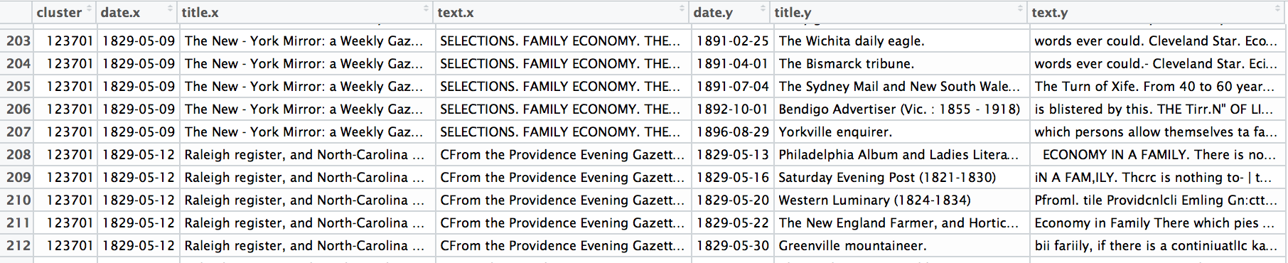
A small example of pairwise data generated by the code above. Each line represents one pair of shared texts between publications. With a few column name changes, such reprinting data becomes network data, with source and target nodes.
The full_join in our code joins our cluster data to itself using the cluster column, which means that it creates a data frame with one line for every potential pair of reprints within each cluster: in other words, we’re creating one line for each potential edge in our network. These lines will include all the columns in the data set for each of the two reprints it now represents; we have created a wide representation of our clusters then, though this process dramatically expands the data frame’s width and length. A cluster of only 5 reprints, for instance, can be paired in 20 unique ways (1-2, 1-3, 1-4, 1-5, 2-1, 2-3, 2-4, 2-5, 3-1, 3-2, 3-4, 3-5, 4-1, 4-2, 4-3, 4-5, 5-1, 5-2, 5-3, 5-4) and many of our clusters are significantly larger than 5. The final step in the code above, however, helps pare down the data set a bit and is rooted in the historical phenomenon we are modeling: exchanges among nineteenth century newspapers. If our model must assume that a shared text between two newspapers is a signal of potential influence, however small, we can also assume such influence only runs forward in time. That is, we likely should not assume that the Daily Dispatch printing a text before the Sunbury American indicates any influence, however small, from the American to the Dispatch, but we might assume the reverse, particularly if Dispatch —> American proves to be a trend, as we will investigate below. The final line of code above, however, filters the data to only those lines in which the date of the first reprint is less than—or, earlier in time than—the date of the second reprint.
From here, we could easily use R to tally raw weight for each edge.
SciAmEdges <- SciAmDirected %>% group_by(title.x,title.y) %>%
  summarize(weight = n())
In short, we would combine each line that lists a given combination of two titles into a single line, tallying a new weight column that increases by 1 for each observation of that combination. So, if in our data frame above there are 42 instances in which the Dispatch printed a text that the American later reprinted, this would result in a single line in our new data frame:
| Source | Target | Weight |
|---|---|---|
| Daily Dispatch | Sunbury American | 42 |
These raw weights give us a baseline from which to test the different lenses I will describe below. One practical reason to strive for better optics, however, is that our data often results in the hairiest of “hairball” network graphs.
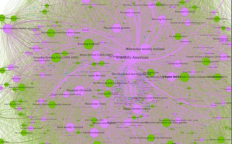
An unfiltered detail of the Scientific American ego network graph. The density of edges makes it difficult to read: this is, in network parlance, a “hairball.”
Because our data is drawn from found connections between papers, our graphs tend to be quite densely connected, even more than I expected going into the Viral Texts Project. That is, I expected more distinct communities that shared texts which did not circulate more widely, while in contrast we are finding that reprinted texts quite often diffused across the exchange system.
Indeed, though we can generate visual graphs in Gephi using our modified network outputs below, we will ultimately be most interested in the values for the weight as they are modified, and how those modified weights change the network statistics for our nodes. Which nodes appear to be most central (or have the highest degree, etc.) when we adjust our weights by time lag, and how do those compare with the nodes that appear to be most central when we adjust our weights by geographic distance, or the edit distance between the versions of the texts they published? Can we triangulate from these three models of our network to discern the links that truly seem indicative of historical connections rather than data artifacts?
Weighing by Publication Lag

“A Curious Calculation,” as it appeared in the Sunbury American and Shamokin Journal (15 May 1847).
While texts circulated among newspapers over many years in the nineteenth-century—indeed, sometimes for decades—they were not typically reprinted steadily through the decades of their lives. Instead, we observe peaks of circulation, fallowness, and recirculation as texts moved in and out of the exchange network. Consider the following graph of cluster 5701252, a scientific-religious tidbit that tries to explain just how big a billion truly is: “For to count a billion, [Adam, having started when created] would require 9,512 years, 34 days, 5 hours, and 20 minutes.” This piece was first printed in Scientific American on April 10, 1847 and printed in at least 175 other publications around the world through at least December 22, 1899. However, if we visualize those reprintings over time through a histogram, we can see the cycles of its publication over time: the largest following its initial publication, another around 1855, for example, and another (following a several years gap) around 1874.

Reprints of Cluster 5701252, or “A Curious Calculation,” plotted over time.
This is a typical pattern for the reprints we have identified: cycles of attention and inattention as a given text moved through exchanges, was forgotten, and was then revived by an editor years later, to echo again through the exchanges, sometimes as if a new text altogether and sometimes with a memory of its earlier circulation. Ideally, we would want to account for these temporal clusterings in our network models, treating jointly reprinted texts nearby in time as stronger potential signals of connections among newspapers than texts reprinted at a long temporal distance. The latter might yet be signals of connection, but our understanding of nineteenth century exchange dynamics suggests it is less likely to be so than those shared texts nearer in time.
In other words, we want to model the network to account for those likelihoods without entirely discounting connections that span larger time gaps. We should not discard edges with a long time lag, but we should treat them as less important individually (though they might yet be important in aggregate). To do this, we can use the following:
SciAmDirected$lag <- SciAmDirected$date.y - SciAmDirected$date.x
SciAmDirected$lagWeight <- 1 / as.numeric(SciAmDirected$lag)
SciAmEdges <- SciAmDirected %>% group_by(title.x,title.y) %>%
  summarize(meanLag = mean(lag), Weight = sum(lagWeight), rawWeight = n())
Here, rather than each shared reprint between two publications increasing the weight of their shared edge by 1, it increases by 1 divided by the lag—measured in days—between each text’s publication in its source and target papers. In other words, the longer the lag in any given pair, the smaller the weight increase for the overall connection. If two publications share a great many texts, even despite a large lag in most instances, the weight of their shared edge will still increase, and the signal of a potential connection will remain. However, it will increase less than it would were the same publications frequently reprinting texts in common near the same time. When we sum up all the edges to create this network model, we retain both a raw weight—the total number of shared reprints for any two publications—as well as a weight adjusted for lag. Looking at the strongest twenty edges as sorted by raw and lag-adjusted weights, we can see how this shifts our view of the network.
As nodes in the network this process produces, these publications will also have stronger calculations for network measures such as degree and centrality. When we factor in publication lag, we might note that publications in New York and New England occupy a good many of the top connections with the New York-based Scientific American: though not all, as the tantalizing (for different reasons) examples of the Milwaukee Weekly Sentinel and Sydney Morning Herald (Australia) show. In the latter case, we can see a stark difference between the raw weight (3967 shared texts in the data set) and the lag-adjusted weight (71.2152435), thanks to a mean lag of 815.18 days between texts being published in Scientific American and appearing in the Sydney Morning Herald. Nonetheless, these publications share so many texts that their connections bears out even when we adjust for lag, which to my mind is a strong indicator of a more than casual link between these two publications that demands further study.
When weighing by lag, the following newspapers have the highest degree, which measures all incoming and outgoing edges for each node in the network:
| Publication | Degree |
|---|---|
| Scientific American | 1034 |
| Milwaukee Weekly Sentinel | 702 |
| The Cleveland Morning Herald | 565 |
| The Universal Gazette | 561 |
| Vermont Chronicle | 552 |
| Bangor Weekly Courier | 495 |
| The Vermont Freeman | 489 |
| Evening Bulletin | 488 |
| New York Evangelist | 484 |
| Maine Farmer | 477 |
When sorted by out degree, the picture changes slightly. Out degree measures only outgoing links, which in this context might signal papers that were frequent sources, rather than receivers, of reprinted texts:
| Publication | Out Degree |
|---|---|
| Scientific American | 542 |
| Milwaukee Weekly Sentinel | 395 |
| The Universal Gazette | 338 |
| The Cleveland Morning Herald | 334 |
| North American and United States Gazette | 300 |
| Vermont Chronicle | 295 |
| Bangor Weekly Courier | 291 |
| New York Evangelist | 270 |
| The Weekly Star | 270 |
| The Vermont Freeman | 261 |
To cite one more metric, we might look at betweenness centrality, which measures how frequently a node appears on the shortest path between the other nodes in the network. The top nodes based on this measure are:
| Publication | Betweenness Centrality |
|---|---|
| Scientific American | 226084.5378 |
| Milwaukee Weekly Sentinel | 47904.08621 |
| Evening Bulletin | 39383.88192 |
| The Universal Gazette | 33650.84385 |
| The Sydney Morning Herald | 28940.72233 |
| The Weekly Star | 27086.2622 |
| Vermont Chronicle | 25770.31755 |
| Boston Investigator | 19331.98607 |
| The Wheeling Daily Intelligencer | 19040.22511 |
| The Cleveland Morning Herald | 17782.64068 |
| Yorkville Enquirer | 17640.67485 |
Were this a full network analysis, we might dig further into these statistics to ascertain why these publications are so measured. We might investigate, for example, whether papers such as the Sydney Morning Herald or Yorkville Enquirer are hubs connecting Australian, US, and/or UK newspapers in our corpora, which might account for their high betweenness scores. For these preliminary experiments, though, we might instead ask how these measurements for a network privileging temporal lag compare with the same measurements for a network that privileges another factor, such as geographic distance.
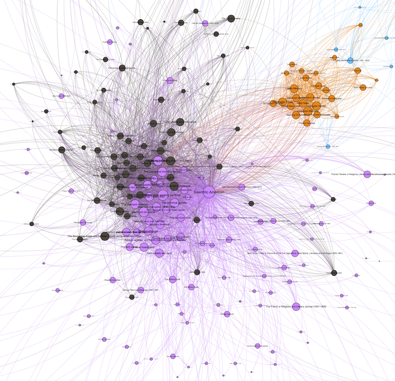
The Scientific American ego network, adjusted for lag, results in more separation and an easier-to-read visualization.
Weighing by Geographical Distance
In some ways, geographic distance has not been as limiting a factor as I expected when we began work on the Viral Texts Project. Newspaper texts circulated around the globe, and far more quickly than I would have anticipated. The “Curious Calculation” article described above was first printed in Scientific American on April 10, 1847, and appeared in a number of UK papers as early as July 3 and Bell’s Life in Sydney and Sporting Reviewer—the earliest Australian reprinting we have identified—on December 4. These are certainly longer spans than we are accustomed to in the internet age, but given the miles and leagues these texts had to travel in the mid-nineteenth century these speeds are impressive.
Nevertheless we do frequently see in our network graphs, as we would expect, more frequent and stronger connections between newspapers nearby geographically than those farther dispersed. In this experiment I privilege and even accentuate those effects by weighing the graph’s edges by physical distance. Here is the pertinent (and no doubt painfully messy) code:
library(dplyr)
library(geosphere)

SciAmSimpleGeo <- select(SciAm, cluster, date, series, title)
#import gazetteer file
gazetteer <- select(read.csv(file = "./geoData/vgaz_out_sorted.csv", header = TRUE), series, latitude, longitude)
#join gazetteer with clusters
SciAmGeo <- left_join(SciAmSimpleGeo, gazetteer, by = "series", match = "all")
#Temporary: omit lines with missing lat/long data
SciAmGeo_complete <- na.omit(SciAmGeo)

#create pairwise data with lat/longs
SciAmGeoPairs <- full_join(SciAmGeo_complete, SciAmGeo_complete, by = "cluster")
#select only edges moving between an older and newer reprinting
SciAmGeoDirected <- filter(SciAmGeoPairs, date.x < date.y)

#calculate geographical distance between papers in each edge
SciAmGeoDirected$edgeDist <- distHaversine(matrix(c(SciAmGeoDirected$longitude.x, SciAmGeoDirected$latitude.x), ncol = 2), matrix(c(SciAmGeoDirected$longitude.y, SciAmGeoDirected$latitude.y), ncol = 2))
#An edgeDist value of 0 (as when 2 papers are printed in the same city) confuses the calculation, so we need to replace those 0 values with 1 so their weights will be unaffected by distance in the adjusted calculation
SciAmGeoDirected$edgeDist[SciAmGeoDirected$edgeDist==0]<-1

#adjust weight for distance
SciAmGeoDirected$distWeight <- 1 / as.numeric(SciAmGeoDirected$edgeDist)
SciAmGeoEdges <- SciAmGeoDirected %>% group_by(title.x,title.y) %>%
  summarize(meanDist = mean(edgeDist), distWeight = sum(distWeight), rawWeight = n())
SciAmGeoEdges$distEffect <- SciAmGeoEdges$rawWeight / SciAmGeoEdges$distWeight
I won’t belabor my explanation this time, as most of these steps echo those above. There are important differences worth explaining, however. First, this code makes use of a gazetteer prepared by Viral Texts RA Thanasis Kinias, which includes the latitude and longitude of most publications in our study (we are currently identifying and adding the few that are missing). I merge that gazetteer with the cluster data by publication IDs, so that each line in the data frame includes the geographic location of the reprinting it describes. Next, this code makes use of the geosphere R library to calculate the physical distance between each pair of reprintings. This distance is calculated as the crow flies, and so is a rather blunt calculation. A more sophisticated version of this experiment might attempt to incorporate what we know about postal roads, railroads, or other communications technologies, but for now we will suffice with a raw measure of distance. As we did with lag in the first experiment, we will modify the weights of each edge, dividing the raw weight of 1 for each instance of a given pairing by the geographic distance between the edge’s two publications.
The resulting network weighed by distance looks quite different from that produced by privileging lag, and its statistics are likewise distinct. In quick succession, here are the top nodes by degree, out degree, and betweenness centrality:
| Publication | Degree |
|---|---|
| Scientific American | 1673 |
| Boston Investigator | 1516 |
| Manchester Times | 1400 |
| New York Evangelist | 1380 |
| The Universal Gazette | 1373 |
| Vermont Chronicle | 1348 |
| Preston Chronicle | 1342 |
| Trewman's Exeter Flying Post | 1335 |
| Hampshire/Portsmouth Telegraph | 1328 |
| Bristol Mercury | 1327 |
| Publication | Out Degree |
|---|---|
| The Universal Gazette | 806 |
| Scientific American | 748 |
| Vermont Chronicle | 741 |
| Bristol Mercury | 721 |
| Liverpool Mercury | 716 |
| Raleigh Register, and North-Carolina Weekly Advertiser | 707 |
| Caledonian Mercury | 705 |
| Boston Investigator | 701 |
| Manchester Times | 698 |
| Preston Chronicle | 696 |
| Publication | Betweenness Centrality |
|---|---|
| Scientific American | 79946.95562 |
| The Universal Gazette | 48036.30927 |
| Hampshire/Portsmouth Telegraph | 34428.81814 |
| Aberdeen Journal | 34312.00833 |
| Boston Investigator | 26266.5412 |
| Liverpool Mercury | 22961.1539 |
| Caledonian Mercury | 19717.94059 |
| Vermont Chronicle | 19436.25648 |
| Bristol Mercury | 18786.61772 |
| Trewman's Exeter Flying Post | 18635.27305 |
Immediately apparent is the spread of this graph: the network is less tightly clustered than previous iterations, separating (as we would expect) into more distinct geographic groups that mostly align with the different, largely nationally organized, corpora from which we are drawing in the Viral Texts Project. What’s perhaps becomes most interesting, then, are those nodes that sit between those geographic communities, which we might hypothesize served as hubs for the international exchange of information. The Aberdeen Journal, for instance, is grouped into a community with other UK newspapers using Gephi’s modularity algorithm, but it also has quite strong ties (despite the long distances) with Australian papers, and clusters near them in the graph. Perhaps unsurprisingly, then, the Aberdeen Journal has one of the highest betweenness centrality measures in the graph, as it may have served as a hub for the movement of texts between the UK and Australian newspaper communities. We would need to do more work with the paper itself to substantiate this hypotheses (or disprove it), but I offer this as one example of how network models point toward new literary-historical research questions.
If our goal is to triangulate among the different network models in our experiments here, we might focus our attention on those publications that appear on both lists: e.g. the Boston Investigator, the New York Evangelist, or the Vermont Chronicle. Certainly publications important in both graphs have a higher likelihood of being important to our overall understanding of the relationships they represent. However, we might just as easily ask about the differences. What does it mean when a publication appears as important in a graph weighted by time and less important in a graph weighted by geographic space? These kinds of questions should guide our refinements to these methods in the coming months.
Weighing by Approximate String Matching
This final investigation is still in progress. I will write a followup post when I have something more concrete to say about how string matching—a kind of computational bibliographic exercise, of collation—might nuance our calculations of weight as lag and distance do above. As a preview, in this experiment I will be estimating the distance between our observed reprinted texts using Levenshtein distance as implemented by the R package stringdist.
Concluding Questions
In closing I offer no conclusions, only questions and provocations. One of our greatest challenges in modeling the networks uncovered through reprinting in Viral Texts has been that our population is so sparse: far more of the network remains invisible than visible, even when drawing from many thousands of digitized newspapers. We must find ways to reflect those gaps in our knowledge in our models of the system, and to supplement our computational work with the insights of literary historical scholarship that can contextualize—and even inform, as I’ve tried to show here—the graphs and visualizations produced by what computation can reveal. Much, much more remains to be done to refine these models and develop effective methods for bringing them into generative conversation. For one, I hope to develop a clear method and rationale for calculating the effects of these modifications: what are the nodes most dramatically affected by adjusting for lag? For distance? For textual difference? From there, we need a clear way to articulate how such faceted graphs intersect, where they diverge, and what those points of intersection and divergence mean for our understanding of the historical relationships they evidence.
Notes
- For more on our reprint detection methods, see our articles in American Literary History (August 2015), Reprinting, Circulation, and the Network Author in Antebellum Newspapers and Computational Methods for Uncovering Reprinted Texts in Antebellum Newspapers.↩ Browse the cluster data I used for these experiments. These are themselves experimental clusters using a new version of the reprint-detection algorithm, and are not yet suitable for formal publication.